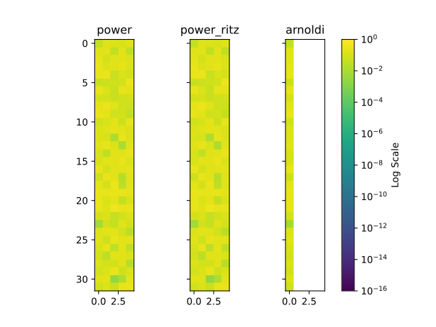
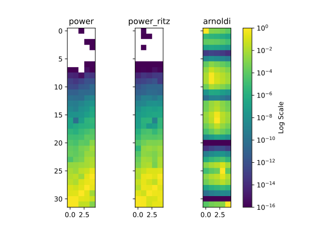
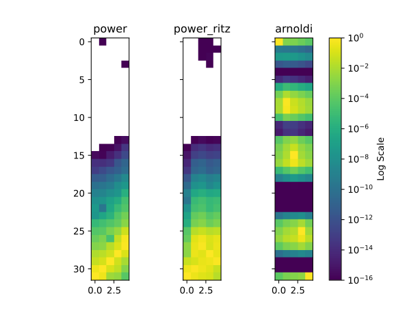
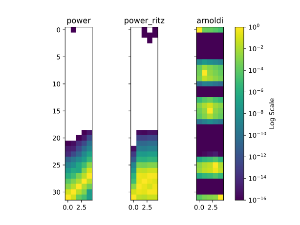
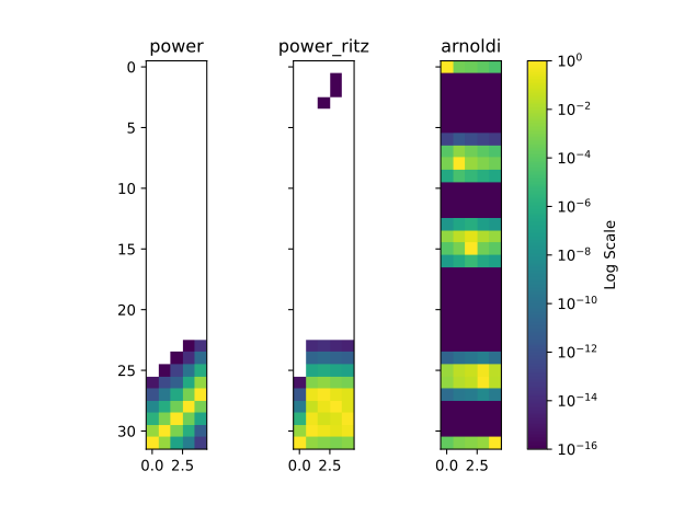
I show a simple illustration of eigensolvers converging on eigenvectors for a very simple case: a diagonal matrix. While the diagonal matrix is a trivial example because we can analytically compute its eigenvalues (diagonal entries) and eigenvectors (columns of the identity matrix), it captures the exact-arithmetic polynomial approximation problem for a symmetric matrix. The fact that we can decompose any symmetric matrix \[ A = V \Lambda V^T \] with orthonormal \(V \) and diagonal \( \Lambda \) means that any polynomial of \(A\) can be fully described by that same polynomial on \( \Lambda \), and since the defining feature of Krylov methods is the use of polynomials this means we can reproduce its spectral convergence behavior with a diagonal matrix and a correspondingly rotated starting vector. Finite-precision behavior and the cost of applying \(A\) are not preserved by this reduction, so the diagonal experiment isolates convergence rather than implementation difficulty.
I show three simple eigensolver prototypes.
This algorithm starts with an orthonormal basis \(V\), applies \( A \) to it, QR factorizes the result, and repeats the process. This is usually called simultaneous iteration or subspace iteration. It uses a QR factorization internally, but it is not the classical QR eigenvalue algorithm that repeatedly factorizes and updates the matrix itself.
import numpy as np
import scipy.linalg as la
from typing import Callable, Optional

def power(
    A: np.ndarray,
    V: np.ndarray,
    maxiter: int = 20,
    callback: Optional[Callable[[np.ndarray], None]] = None
) -> np.ndarray:
    """
    Power iteration-like method for refining an orthonormal basis.

    This algorithm starts with an initial orthonormal matrix `V`, applies `A` to it,
    then performs a QR factorization, repeating this process for `maxiter` iterations.

    Args:
        A (np.ndarray): The matrix to be applied iteratively.
        V (np.ndarray): Initial orthonormal basis.
        maxiter (int, optional): Number of iterations to run. Default is 20.
        callback (Optional[Callable[[np.ndarray], None]], optional):
            A function that is called with `V` at each iteration. Default is None.

    Returns:
        np.ndarray: The final orthonormal matrix after iterations.
    """

    # Ensure V is an orthonormal basis initially
    V, _ = la.qr(V, mode="economic")

    # Call the callback with the initial V if provided
    if callback:
        callback(V)

    # Iterative process
    for _ in range(maxiter):
        AV = A @ V  # Apply matrix A to V
        V, _ = la.qr(AV, mode="economic")  # Re-orthonormalize using QR factorization

        # Call the callback function at each iteration if provided
        if callback:
            callback(V)

    return V
By doing a little extra work on each iteration of the QR iteration we can compute Ritz vectors which provide eigenvector approximations from the subspace represented by \( V \)
import numpy as np
import scipy.linalg as la
from typing import Callable, Optional

def power_ritz(
    A: np.ndarray,
    V: np.ndarray,
    maxiter: int = 20,
    callback: Optional[Callable[[np.ndarray], None]] = None
) -> np.ndarray:
    """
    Power iteration with Ritz vector refinement.

    This algorithm iteratively applies `A` to an orthonormal basis `V`,
    performs QR factorization, and refines the basis using the eigenvectors
    of the projected matrix `V^T A V`.

    Args:
        A (np.ndarray): The matrix to be applied iteratively.
        V (np.ndarray): Initial orthonormal basis.
        maxiter (int, optional): Number of iterations to run. Default is 20.
        callback (Optional[Callable[[np.ndarray], None]], optional):
            A function that is called with `V` at each iteration. Default is None.

    Returns:
        np.ndarray: The final orthonormal matrix after iterations.
    """

    # Ensure V is an orthonormal basis initially
    V, _ = la.qr(V, mode="economic")

    # Call the callback with the initial V if provided
    if callback:
        callback(V)

    # Iterative process
    for _ in range(maxiter):
        AV = A @ V  # Apply matrix A to V
        V, _ = la.qr(AV, mode="economic")  # Re-orthonormalize using QR factorization

        # Compute the Rayleigh quotient for the *new* basis: VTAV = V^T A V
        VTAV = V.T @ A @ V

        # Solve for eigenvalues and eigenvectors of VTAV
        eigenvalues, W = la.eigh(VTAV)

        # Transform V using the Ritz vectors
        V = V @ W

        # Call the callback function at each iteration if provided
        if callback:
            callback(V)

    return V
The next algorithm breaks from the previous algorithms by not driving all vectors in \( V\) at the same time. This leads to economy of evaluations of \(Ax\) but creates a data dependency in between every such evaluation, making it impossible to batch them. The payoff is high convergence rates.
This algorithm also orthogonalizes in between steps but does so through the Arnoldi factorization instead of the QR factorization: \(A V_k = V_{k+1}\bar H_k\), where \( V_{k+1} \) is orthonormal and \( \bar H_k \) is upper Hessenberg.
import numpy as np
import scipy.linalg as la
from typing import Callable, Optional

def arnoldi(
    A: np.ndarray,
    v: np.ndarray,
    k: int,
    maxiter: int,
    callback: Optional[Callable[[np.ndarray], None]] = None
) -> None:
    """
    Arnoldi iteration for Krylov subspace approximation.

    This algorithm constructs an orthonormal basis of the Krylov subspace using
    the Arnoldi process and computes the Hessenberg matrix `H`. It refines the
    basis using eigenvectors of `H` at each iteration.

    Args:
        A (np.ndarray): The matrix for which the Krylov subspace is constructed.
        v (np.ndarray): The initial vector for Krylov subspace iteration.
        k (int): The number of Arnoldi iterations to perform per cycle.
        maxiter (int): The total number of iterations.
        callback (Optional[Callable[[np.ndarray], None]], optional):
            A function that receives the orthonormal basis at each iteration. Default is None.

    Returns:
        None: The function does not return a value but may call `callback` at each step.
    """

    # Utility functions for norm and dot product
    norm = np.linalg.norm

    m = v.size  # Dimension of the vector space
    V = np.zeros((m, k + 1))  # Orthonormal basis matrix
    H = np.zeros((k + 1, k))  # Upper Hessenberg matrix

    # Normalize initial vector
    V[:, 0] = v / norm(v)

    # Call the callback function with the initial basis if provided
    if callback:
        callback(V[:, :k])

    nevals = 0  # Number of evaluations
    while nevals < maxiter:
        # Re-normalize the starting vector at the beginning of each cycle
        V[:, 0] = v / norm(v)

        for j in range(k):
            w = A @ V[:, j]  # Apply A to the current basis vector
            h = V[:, :j + 1].T @ w  # Project w onto existing basis in V

            # Compute residual f after projection
            f = w - V[:, :j + 1] @ h
            # "DGKS" correction
            s = V[:, :j + 1].T @ f
            f -= V[:, :j + 1] @ s
            h += s

            beta = norm(f)  # Compute norm of f
            H[:j + 1, j] = h  # Store coefficients in H
            H[j + 1, j] = beta  # Subdiagonal value

            if beta == 0.0:
                raise RuntimeError("Arnoldi breakdown: invariant subspace found")
            V[:, j + 1] = f / beta  # Normalize and store new basis vector

        nevals += k  # This cycle used k matrix-vector products

        # Compute eigenvalues and eigenvectors of the Hessenberg matrix
        eigenvalues, W = la.eigh(H[:k, :k])  # Valid here because A is symmetric

        # Call the callback function with the transformed basis if provided
        if callback:
            callback(V[:, :k] @ W)

        # Update the starting vector for the next cycle
        v = V[:, :k] @ W @ np.ones(k)
The matrix I use just contains positive real diagonal values starting at \(r>0\) and ending at \(1\).
For visualization purposes I use a small matrix with just 32 rows, and I ask each eigensolver to compute \(k=5\) eigenvectors.
The Arnoldi prototype was initialized with a random vector with uniformly distributed entries; the subspace iterations require a random matrix with \(k\) columns, which is orthonormalized before the first step.
The original plots label a full update of the displayed basis as an “iteration,” but that is not a fair unit of work: one subspace-iteration step applies \(A\) to \(k\) vectors and one Arnoldi cycle also performs \(k\) sequential matrix-vector products. Matrix-vector product count, together with orthogonalization cost, is the cleaner comparison.
Finally to visualize I show the state of each iteration for the computed eigenvectors. Since the matrix is diagonal we know the eigenvectors are just columns of the identity matrix, so we know that the eigenvectors should converge to just one nonzero entry. None of these algorithms attempt any kind of shift, deflation, or careful restarting that would allow us to select specific eigenvalues so the only thing they will do is converge to some eigenvectors
| Iteration | Computed Eigenvectors |
|---|---|
| 0 | |
| 25 | |
| 50 | |
| 100 | |
| 200 | |
Subspace iteration, as expected, converges to the invariant subspace associated with the eigenvalues of largest magnitude. The original Ritz-vector version appeared to have trouble converging to individual identity columns because its projected matrix mixed the newly computed basis \(V\) with the stale product AV from the previous basis. The corrected code recomputes V.T @ A @ V. Ritz rotation does not change the converged subspace, but it should turn a sufficiently accurate invariant subspace into individual eigenvector approximations when the selected eigenvalues are distinct.
The most interesting result here for me was the Arnoldi iteration, which produced Ritz vectors from a wider part of the spectrum rather than only the largest eigenvalues. This prototype uses a simple explicit restart by summing the current Ritz vectors, so the pictures show that particular heuristic rather than a standard implicitly restarted Arnoldi method.