Here I look at “Compensated” arithmetic and its application to a small side-project CompensatedBLAS. Compensated arithmetic allows you to implement higher-accuracy accumulation using expansions of lower-precision floating-point words. Two FP32 words carry at most roughly 48 significand bits before nonoverlap and implementation losses, so they do not in general reproduce the 53-bit significand or correctly rounded behavior of FP64. More expansion terms can approach or exceed FP64 accuracy, but this requires a careful error analysis. This approach to higher-accuracy calculation has advantages over simply copying all data to a higher working precision and then doing arithmetic there. First it is often the case that only a very small number of values actually need the higher precision treatment, thus your input data can remain in the lower working precision without need to copy it into a higher working precision. Secondly it is sometimes the case that an architecture may handle the lower precision words fundamentally much faster than the higher precision words. Examples of this are tensor cores on many NVIDIA GPUs that accelerate lower-precision inputs substantially, although supported input and accumulation precisions depend on the tensor-core generation and instruction mode. On many CPUs there is no instruction that takes FP32 operands and accumulates an FMA directly into FP64 lanes; explicit conversion reduces SIMD width and adds instructions. With all of the above in mind, compensated arithmetic lets input data remain in a working precision while backend code trades additional lower-precision operations and storage for a chosen number of expansion terms. It does not provide arbitrary precision for free. I end the post with concrete examples of compensated accumulations improving pathological numerical behavior in particular when it involves repeated calls into BLAS routines where we accumulate into the same matrix repeatedly.
Compensated arithmetic starts with the idea of expanding a single floating-point value into one primary word plus k compensation words each representing a different exponent range.
1) EXPANSION (ONE PRIMARY WORD PLUS k COMPENSATION WORDS)
---------------------------------------------
 true value  ─────────────────────────────────────────►

 [ w0 ] [ w1 ] [ w2 ] ... [ wk ]
   ▲       ▲     ▲           ▲
   |       |     |           |
 highest   next  finer ...   finest kept bits
 word      spill spill        (beyond this are dropped)

- Each wi is a normal floating-point word. The sum w0 + w1 + ... + wk-1 ≈ true value.
- w0 carries most magnitude; bins w1..wk-1 store progressively tinier “lost” bits.
Initially the k compensation words are zero. Suppose we have a way to represent a floating-point sum as a rounded primary word plus its exact residual. Call this two_sum, so that [x,e] = two_sum(a,b) represents a+b with two words. We can then cascade residuals through an arbitrary fixed number of compensation words. Increasing k retains more information, subject to overflow, underflow, nonoverlap, and final-rounding details:
B) CASCADED INSERTION OF ONE VALUE x
------------------------------------
Goal: add x into (w0..wk-1) using only two_sum.

function insert(x):
  (w0, c) = two_sum(w0, x)   // c = spill from adding x into w0
  (w1, c) = two_sum(w1, c)   // pass spill down the stack
  (w2, c) = two_sum(w2, c)
   ...
  (wk-1, c) = two_sum(wk-1, c)
  // leftover c would be kept if we had more bins

Flow:

  x ──► [two_sum] ──► w0'   carry c0 ─► [two_sum] ─► w1'
                                       c1 ─► [two_sum] ─► w2'
                                                ...
                                      ck-2 ─► [two_sum] ─► wk-1'
This is the core idea of compensated arithmetic, and this is the theme that plays out repeatedly. Now I show concretely how to implement two-sum and two-prod (for products).
Under round-to-nearest IEEE arithmetic and absent exceptional overflow/underflow behavior, two_sum exactly represents the sum of two floating-point words a,b with two floating point words of the same length. In C++ this can be implemented as follows
// ---------------------------------------------
// two_sum: error-free transform of a+b
// Returns (s, e) with s = fl(a+b) and a + b = s + e exactly.
// Reference: Knuth’s 2Sum.
// ---------------------------------------------
inline std::pair<double, double> two_sum(double a, double b) {
    double s  = a + b;              // Rounded sum
    double bp = s - a;              // Portion of s contributed by b
    double e  = (a - (s - bp)) + (b - bp);  // Recover lost low bits
    return {s, e};
}
The compiler must preserve the sequence of rounded operations in an error-free transform. Aggressive reassociation or fast-math transformations can invalidate the proof, so these kernels need appropriate floating-point compiler settings.
and a diagram to help visualize
2) HOW two_sum(a,b) CAPTURES LOST ADDITION BITS
-----------------------------------------------
 Let s = fl(a+b), e = exact_low_bits so that a + b = s + e exactly.

       exponent axis (coarse) →  [ ...  2^E  ...  2^(E-52) ... ]
 a:    |==========mantissa bits===========|
 b:                    |======mantissa=======|
 s:    |==========rounded to 53 bits===========|
 e:                           |residual|

- s is the rounded result in working precision.
- e is the “spill” that didn’t fit in s’s mantissa window.
- We insert s into w0, and cascade e into bins w1.., preserving information.
Numerical linear algebra mostly deals in dot products or axpy-like operations though, which means we also need products. Fortunately there is an equivalent two_prod for products
Subject to the same finite-value and underflow qualifications, two_prod, like two_sum, represents the product of a*b with two floating-point words of the same length as the inputs. In architectures with fused-multiply-add we can implement this fairly efficiently like below
// ---------------------------------------------
// two_prod: error-free transform of a*b using FMA
// Returns (p, e) with p = fl(a*b) and a*b = p + e exactly.
// ---------------------------------------------
inline std::pair<double, double> two_prod(double a, double b) {
    double p = a * b;               // Rounded product
    double e = std::fma(a, b, -p);  // Exact residual from FMA
    return {p, e};
}
The key to the fused-multiply-add isn’t just that it combines operations efficiently, but specifically that it rounds only once at the end.
4) HOW two_prod(a,b) CAPTURES LOST MULTIPLICATION BITS
------------------------------------------------------
 two_prod(a,b) returns p,e with a*b = p + e exactly (using FMA).

mantissa windows (concept):

 a:  |==========|
 b:  |==========|
 p:  |==========rounded  a*b|==========|
 e:                         |low part from FMA|

- Insert p then e into the expansion to keep product bits beyond 53 bits.
Combining two_sum, two_prod and k-term accumulation we get a core linear algebra kernel: the dot product
// -----------------------------------------------------------
// k_term_compensated_dot:
//   Computes sum_i x[i]*y[i] using a k-term compensated accumulator.
//   Holds one main term and k side terms (approx. k+1-word precision).
//
// Parameters:
//   x, y : input arrays
//   n    : length
//   k    : number of compensation terms
//
// Notes:
//   * Loops could early-exit if r==0.0, but we skip that for simplicity.
//   * Final reduction uses long double when it is wider than double.
// -----------------------------------------------------------
inline double k_term_compensated_dot(const double* x,
                                     const double* y,
                                     std::size_t n,
                                     int k)
{
    double main = 0.0;
    std::vector<double> comp(k, 0.0);

    for (std::size_t i = 0; i < n; ++i) {
        // Multiply exactly
        auto [p, pe] = two_prod(x[i], y[i]);

        // Insert p into expansion
        auto [new_main, r] = two_sum(main, p);
        main = new_main;
        for (int j = 0; j < k; ++j) {
            auto [new_cj, r2] = two_sum(comp[j], r);
            comp[j] = new_cj;
            r = r2;
        }

        // Insert product residual pe
        auto [new_main2, r3] = two_sum(main, pe);
        main = new_main2;
        for (int j = 0; j < k; ++j) {
            auto [new_cj, r4] = two_sum(comp[j], r3);
            comp[j] = new_cj;
            r3 = r4;
        }
    }

    // Fold expansion in the implementation's long-double precision
    long double hi = static_cast<long double>(main);
    for (int j = 0; j < k; ++j)
        hi += static_cast<long double>(comp[j]);

    return static_cast<double>(hi);
}
The final long double fold is a convenience rather than a portable guarantee of correct rounding: on some platforms long double is identical to double. A correctly rounded BLAS would need an explicit final-rounding strategy.
With the above we can implement actually a huge number of BLAS routines, which I have done in CompensatedBLAS.
CompensatedBLAS is a small project I made to implement BLAS with three goals:
LD_PRELOAD the CompensatedBLAS library without changing the application)The BLAS ABI still has to match the application’s integer width and symbol conventions. The project is early and has not fully implemented BLAS yet, but has a good amount ready.
This behavior is what you would see if you simply linked CompensatedBLAS into an existing project and started to use it. It accumulates into k compensation terms and computes the rounded result in working precision at the end of the call.
#include "compensated_blas.hpp"
#include <vector>
#include <iostream>

extern "C" {
double ddot_(const long long* n, const double* x, const long long* incx,
             const double* y, const long long* incy);
}

int main() {
  using namespace compensated_blas::runtime;
  set_compensation_terms(0);  // plain accumulation

  std::vector<double> x{1.0, 1e-16, -1.0};
  std::vector<double> y{1.0, 1.0, 1.0};
  const long long n = (long long)x.size(), inc = 1;

  double d = ddot_(&n, x.data(), &inc, y.data(), &inc);
  std::cout << "plain ddot = " << d << "\n";
}
If you’re willing to break from a pure BLAS interface you can “register” a vector or a matrix with the CompensatedBLAS runtime and when you pass the associated pointer into routines that will accumulate into it then they will use a k-term expansion that is persisted between calls. Thus you can do thousands of accumulations with e.g. xSYRK or xAXPY and still round only once at the end. In this case rounding is explicitly the caller’s responsibility, so this is definitely not typical BLAS behavior but it is useful to expose to users.
#include "compensated_blas.hpp"
#include <vector>
#include <iostream>

extern "C" {
void daxpy_(const long long* n, const double* alpha, const double* x,
            const long long* incx, double* y, const long long* incy);
}

int main() {
  using namespace compensated_blas::runtime;
  set_compensation_terms(1);                 // enable 1 bin
  clear_deferred_rounding_registrations();  // start clean

  std::vector<double> x{1.0, 1e-16, -1.0};
  std::vector<double> y{0.0, 0.0, 0.0};

  // Register the *output* so its per-element bins are kept (deferred rounding).
  deferred_rounding_vector_t desc{};
  desc.data = y.data(); desc.length = y.size(); desc.stride = 1;
  desc.element_size = sizeof(double); desc.alignment = alignof(double);
  desc.type = scalar_type_t::real64;
  register_deferred_rounding_vector(desc);

  const long long n = (long long)x.size(), inc = 1;
  const double alpha = 1.0;
  daxpy_(&n, &alpha, x.data(), &inc, y.data(), &inc);   // y += x (with bins)

  // Schematic: flush here, using the runtime's finalization helper, before
  // reading y or clearing its registration. That folds the bins into y.

  std::cout << "y[0..2] after daxpy (deferred, 1 term): "
            << y[0] << ", " << y[1] << ", " << y[2] << "\n";

  clear_deferred_rounding_registrations();
  set_compensation_terms(0);  // back to plain mode if desired
}
For the most part applying compensation to BLAS amounts to finding efficient ways to roll the compensated dot product above into the inner loops of ordinary BLAS. For example we may want the k compensation terms to be laid out in memory strided rather than contiguously so that we can vectorize the two-sum & two-prod with the same stride that the underlying BLAS is vectorized.
The primary exceptions to this are givens rotations and triangular solves with non-unit diagonals. My first attempt in CompensatedBlas to implement the triangular solves involved a somewhat clumsy Newton-Raphson refinement of division to expand it out to k terms. In retrospect I think it would be better to block the triangular solve into small sub-matrix triangular solves (small enough that compensation terms can be static arrays embedded in the function) and then do iterative refinement on each sub-matrix solve, using compensated matrix-matrix/vector product for the residual.
For Givens rotations I did not put much effort beyond simply getting the Netlib BLAS test suite to pass. This is not a statement about the general importance of Givens rotations, but rather my own lack of use of them through BLAS.
I came up with two examples where the deferred rounding capability of CompensatedBLAS can improve numerical behavior on common numerical linear algebra algorithms. In both cases these involve repeated calls to BLAS, which means that incorrect roundings on each call accumulate over time resulting in drift away from correct results.
The demo builds an n x n matrix C with n=--size, starting from zeros, by repeating --updates times: generate A with k=--rank columns where each column is a scaled copy of one of --basis cached “dependent” columns plus noise of size --noise-scale that shrinks each step by --noise-decay (randomness fixed by --seed); then do a lower-triangle SYRK update C += A*A^T (alpha=1, beta=1). Two runs are compared: a plain accumulation and a rolling-compensated one that keeps --compensation-terms extra bins per C[i,j] with deferred rounding, flushed at the end. Results optionally dump to --dump-prefix_plain.txt and --dump-prefix_compensated.txt, then the code symmetrizes C and reports the minimum Cholesky pivot as the stability/definiteness metric.
The basic idea of the above experiment is that we repeatedly accumulate rank-k symmetric updates from related vectors so that they aren’t quite linearly dependent, but are almost, and we keep repeating this summation. Eventually without compensation we obtain a good number of negative eigenvalues and a large negative cholesky pivot. Compensation mitigates this significantly though it should be noted that perfectly retaining definiteness on this algorithm will always be limited with a fixed working precision. Compensation bounds the pathological behavior to a very small region in this run, whereas without compensation it grows much larger.
reidatcheson@pop-os:~/clones/CompensatedBLAS/build/examples$ ./syrk_compensation_demo --size=64 --rank=16 --updates=1000 --compensation-terms=4 --dump-prefix=$PWD --seed=0 --basis=64 --noise-scale=3e-4 --noise-decay=0.1
SYRK compensation demo with size=64 rank=16 updates=1000
Plain min Cholesky pivot:        -0.0000045109
Rolling-compensated min pivot:  0.0000019407
(...)

(uncompensated)
Smallest 5 eigenvalues:
  -1.9427982037878256e-12
  2.4192337217676416e-12
  3.9206022117119458e-12
  6.18032870190732e-12
  9.0801014748812597e-12

(compensated)
Smallest 5 eigenvalues:
  7.3348222192768711e-13
  1.3501303405426835e-12
  2.5594292350820926e-12
  5.1230056487681293e-12
  8.5714895623300911e-12
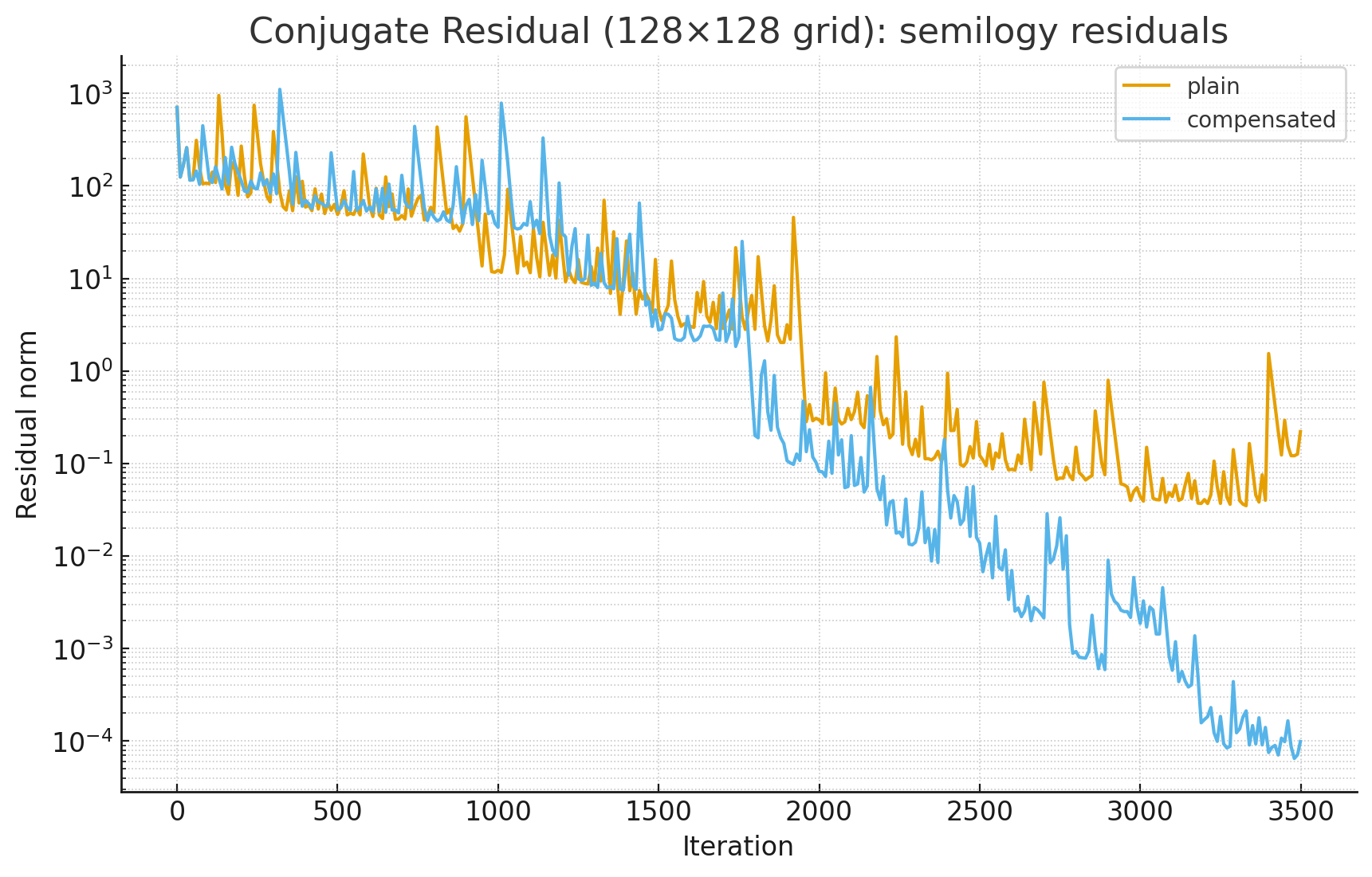
We solve A x = b on a --grid x --grid lattice where A is the 5-point Laplacian (applied with apply_laplacian) and b is all ones, starting from x=0. The implementation used the following short recurrence: at each iteration compute ap = A p, step x += alpha p, r -= alpha ap with alpha = (r·r)/(ap·ap), form ar = A r, then update directions with beta = (ar·ap)/(ap·ap), p = r + beta p, and ap = ar + beta ap. Stop when ||r|| < --tol or after --max-iter; log residual and orthogonality to r0 every --log-interval. Two runs are compared: a plain run and a compensated run that registers x, r, p, ap, ar for deferred rounding with --compensation-terms bins per element (using compensated ddot/daxpy), flushing bins where needed and at the end.
There is an important correction to make here: despite the executable name and my original description, this is not the classical Conjugate Residual recurrence. Classical CR uses r dot (A r) in the step numerator, not r dot r. Thus the data below show that deferred rounding substantially changed this nonstandard recurrence, not that it improved CR.
That is still an interesting observation, but the mechanism is unresolved. The obvious follow-up is to correct the recurrence and track the true residual and relevant orthogonality measures.
reidatcheson@pop-os:~/clones/CompensatedBLAS/build/examples$ ./conjugate_residual_solver --grid=128 --max-iter=3500 --log-interval=500 --compensation-terms=2
Conjugate Residual solver on 128x128 grid (16384 unknowns)
max iterations=3500 tolerance=1e-10 log interval=500
[plain] iterations=3500 final_residual=0.221156
    orthogonality to r0:
      iter=     0 residual=       707.349
      iter=   500 residual=         49.17
      iter=  1000 residual=         12.27
      iter=  1500 residual=       4.60787
      iter=  2000 residual=      0.296416
      iter=  2500 residual=      0.122486
      iter=  3000 residual=     0.0439887
      iter=  3499 residual=      0.221156

[compensated] iterations=3500 final_residual=9.88736e-05
    orthogonality to r0:
      iter=     0 residual=       707.349
      iter=   500 residual=       55.1866
      iter=  1000 residual=       35.7823
      iter=  1500 residual=        2.7677
      iter=  2000 residual=     0.0822101
      iter=  2500 residual=     0.0137711
      iter=  3000 residual=    0.00186914
      iter=  3499 residual=   9.88736e-05
Here is the same set of residuals but sampled every 10 iterations, on a plot.
CompensatedBLAS is still an experimental project, but the SYRK example already gives a concrete case where deferred rounding is useful. The iterative-solver example needs to be rerun with the corrected recurrence. The real question is whether this can be done without a performance tradeoff large enough to kill its utility. I think the answer is ultimately yes, but designing good compensated BLAS microkernels would be highly nontrivial compared with simply implementing naive BLAS as I have done here.