I demonstrate a family of sparse matrices with exactly the same sparsity pattern, same number of rows and columns, good numerical properties but nevertheless perform very differently from each other when factorized using the same sparse LU factorization algorithm. Sparse LU factorizations results in efficient and accurate solution to system of linear equations even with a nonsymmetric underlying sparse matrix. Unlike the Cholesky and QR factorizations however, LU potentially requires pivoting for numerical stability. For the dense case this pivoting does not really impact performance except for very large matrices. For the sparse case however pivoting can introduce extra fill-in - this means more FLOPS necessary to complete and larger memory footprint. I show the construction of the family of sparse matrices using simple Python, SciPy, and NumPy. I then pull 6 matrices from this family and factorize them using scipy.sparse.splu which relies on the SuperLU library. I measure wall clock time and memory usage for each run and show how they differ. I run each factorization 100 times and report statistics to try and control for nondeterministic performance caused by Python garbage collection and parallelism in the SuperLU library.
I use a very simple matrix family to show this performance variation. Starting with the classic 2D Laplacian operator as a sparse matrix \( \mathbf{A} \) (output by function lap2d below), and then scale it by a diagonal matrix as follows \( \mathbf{D}\mathbf{A} \) such that the diagonal entries of \( \mathbf{D} \) span multiple orders of magnitude. For example in the scaling function below has parameter nmags=2 then the diagonal entries of \( \mathbf{D} \) come from the interval \( [1,100] \) and for nmags=3 they draw from the larger interval \( [1,1000] \), and so on. I use a fixed seed for randomly choosing the diagonal entries of \( \mathbf{D} \) for reproducibility.
Note that all matrices have the same size, using mx=my=512 to construct the initial 2D Laplacian sparse matrix.
import numpy as np
import scipy.sparse as sp
import scipy.sparse.linalg as spla
#1D laplacian matrix
def lap1d(m):
    return sp.lil_matrix(sp.diags((np.ones(m),-2.0*np.ones(m),np.ones(m)),(-1,0,1),shape=(m,m)))
#2D laplacian matrix constructed as kroneckor products of 1D laplacian
def lap2d(mx,my):
    Ix=sp.eye(mx)
    Iy=sp.eye(my)
    Lx=lap1d(mx)
    Ly=lap1d(my)
    return sp.kron(Ix,Ly)+sp.kron(Lx,Iy)
#Scale an input matrix with a diagonal matrix
#whose diagonal entries span multiple orders of magnitude,
#specified by the `nmags` parameter
def scaling(A,nmags=2):
    (m,n)=A.shape
    #Use same seed for reproducibility
    np.random.seed(2304814)
    diag=np.random.choice(np.logspace(0,nmags,m),m)
    D=sp.diags(diag,shape=(m,n))
    return D@A
I draw 6 matrices from the family described above (using parameter nmags=1,2,3,4,5,6), run a sparse LU factorization 100 times and report statistics to try and control for nondeterministic performance caused by Python garbage collection and parallelism in the SuperLU library.
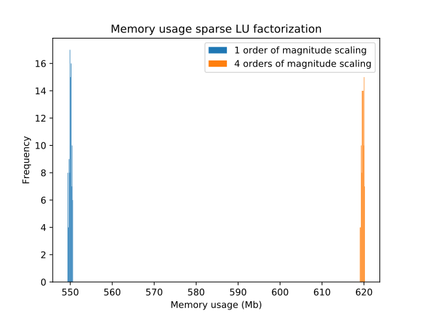
First I show a histogram of 2 of these matrices’ memory usage in SuperLU to illustrate that the histograms are quite well separated and so the difference in memory usage unlikely resulting from other sources of nondeterminism like garbage collection.
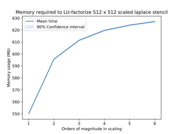
Next I plot the mean memory usage across all 100 runs for each paramter nmags=1,2,3,4,5,6. I also show 99% confidence intervals in this plot but they are small and so not easily seen.
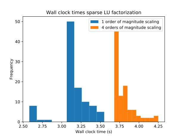
Next I show a histogram of 2 of these matrices and their corresponding wall-clock time in SuperLU. This is to show how well separated the histograms are to rule out other causes of timing differences such as from threading runtime, OS jitter, caching differences between runs, etc.
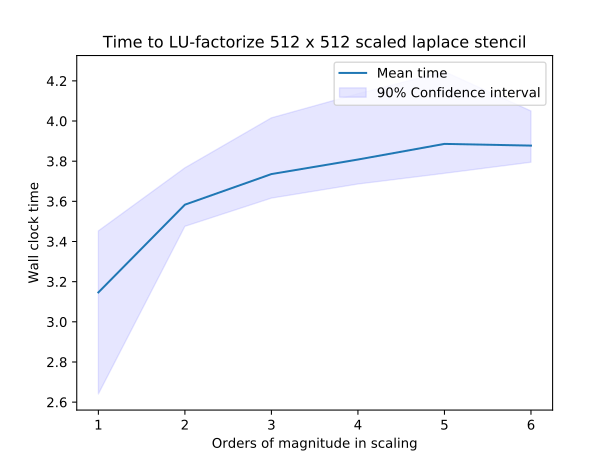
Next I plot the mean wall-clock time across all 100 runs for each paramter nmags=1,2,3,4,5,6. I also show 90% confidence intervals in this plot. The variation in timing between runs was much higher than for memory so these confidence intervals are larger.
I demonstrate a family of matrices that are otherwise numerically well-behaved, very similar to each other, and yet perform very differently when factorized with a sparse LU factorization. The need for pivoting likely caused this performance variation because of the numerical difference between matrices in this family. Algorithms like Cholesky or QR usually do not present with similar variation because they do not similarly need pivoting - although they have their own limitations. This variation in LU has in part led me to further investigate sparse QR factorization to see if I can produce a sparse factorization with reliable memory usage and performance characteristics while addressing some of the shortcomings of QR factorization.