Nightmare Matrices 2: Symmetric Positive Definite Case

I present here a deliberately unpleasant family for sparse linear solvers that operate only on an input sparse matrix. This counter-example is closely related to the nightmare matrices of a previous post, but with a key strengthening: the matrices I present here will be symmetric and positive definite (“SPD” for short). In my prior post I relied on indefiniteness of the matrix to make iterative solutions a non-viable “shortcut” around direct methods. It remained an open question to me whether the expander symbolic structure of a nightmare matrix could even admit an SPD formulation that remains difficult to solve.

The reason it is not obvious is that the standard archetype, the graph Laplacian, often has a favorable nonzero spectrum on an expander. After handling its constant nullspace, this is usually a good situation for Krylov methods. So the open question to me was whether I could force a much less favorable spectral distribution while still preserving SPD and underlying expander structure? The answer turns out to be yes. The construction below gives matrices with the following properties:

1. Sparse: \( O(1) \) nonzeros per row.
2. Symmetric and positive definite
3. Quadratic-looking factor storage in the experiments below
4. A prescribed spectral interval and condition number after scaling the original block
5. Half of the eigenvalues placed at Chebyshev nodes in that interval, producing a difficult CG example

Such a matrix is expensive for sparse direct methods because of excessive fill, while unpreconditioned CG is slow because of the planted spectrum. The obvious weakness is that recognizing the block transform immediately gives a good solver.

I will describe the construction, give numerical results confirming the above properties, and then I’ll give some mitigations a sparse solver library could potentially adopt to overcome my construction although I suspect the approach here could be strengthened to make this prohibitively expensive.

The Construction

The construction works by taking an initial SPD matrix with underlying expander structure and embedding it into a larger matrix that preserves the expander structure but has an enforced spectral distribution to make solving it with Krylov methods difficult.

Suppose \(A_0\in\mathbb{R}^{n\times n}\) is a symmetric positive definite matrix. Then define

And then take the orthogonal block matrix

and set

Equivalently,

If \( A_0 \) is sparse, symmetric, and positive definite then so is \( M \), because it is an orthogonal similarity of the SPD block diagonal matrix. \(M\) is twice as large as \(A_0\) and, up to diagonal coincidences or cancellation, has about twice as many structural nonzeros per row. By appropriately selecting \( D \) we can explicitly specify half of the spectrum. In fact, the spectrum of \(M\) is the union of the spectrum of \(A_0\) and the diagonal entries of \(D\). To claim a prescribed interval [lo,hi] or condition number, the spectrum of A0 must first be scaled into the same interval and the union must attain the desired endpoints.

In words this is reversing a block orthogonal decomposition where our starting point contains the planted eigenvalues as well as an expander matrix.

Sample Code

The following code can compute \(M \) given an \( A_0 \)

import numpy as np
import scipy.sparse as sp
import scipy.sparse.linalg as spla


def chebyshev_nodes(n, lo, hi, *, sort=True):
    """
    First-kind Chebyshev nodes mapped to [lo, hi].

    These are dense near both endpoints but do not include the endpoints.
    """
    j = np.arange(n, dtype=float)
    x = np.cos((2 * j + 1) * np.pi / (2 * n))
    vals = 0.5 * (lo + hi) + 0.5 * (hi - lo) * x
    return np.sort(vals) if sort else vals


def estimate_extreme_eigs_spd(A, *, dense_cutoff=512, tol=1e-8):
    """
    Estimate lambda_min and lambda_max of a real symmetric sparse SPD matrix.

    For small matrices, this uses dense eigvalsh for reliability.
    For larger matrices, this uses scipy.sparse.linalg.eigsh.
    """
    A = sp.csr_matrix(A)
    n, m = A.shape
    if n != m:
        raise ValueError("A must be square.")

    if n <= dense_cutoff:
        vals = np.linalg.eigvalsh(A.toarray())
        return float(vals[0]), float(vals[-1])

    lmin = spla.eigsh(
        A,
        k=1,
        which="SA",
        return_eigenvectors=False,
        tol=tol,
    )[0]

    lmax = spla.eigsh(
        A,
        k=1,
        which="LA",
        return_eigenvectors=False,
        tol=tol,
    )[0]

    return float(lmin), float(lmax)


def planted_spd_lift(
    A0,
    planted_eigs,
    *,
    fmt="csr",
    check_symmetric=True,
    symmetry_tol=1e-10,
):
    """
    Given an n x n sparse SPD matrix A0 and n positive target eigenvalues,
    build a 2n x 2n sparse SPD matrix M whose spectrum is

        spectrum(M) = spectrum(A0) union planted_eigs.

    The construction is

        M = 1/2 [[A0 + D, A0 - D],
                 [A0 - D, A0 + D]]

    where D = diag(planted_eigs).

    The planted eigenvectors are exactly

        [e_i; -e_i] / sqrt(2),

    with eigenvalue planted_eigs[i].

    The original eigenvectors v of A0 lift to

        [v; v] / sqrt(2).
    """
    A0 = sp.csr_matrix(A0)
    n, m = A0.shape

    if n != m:
        raise ValueError("A0 must be square.")

    if check_symmetric:
        diff = (A0 - A0.T).tocoo()
        sym_err = 0.0 if diff.nnz == 0 else float(np.max(np.abs(diff.data)))
        if sym_err > symmetry_tol:
            raise ValueError(
                f"A0 does not look symmetric; max |A0 - A0.T| = {sym_err:g}."
            )

    planted_eigs = np.asarray(planted_eigs, dtype=float)

    if planted_eigs.shape != (n,):
        raise ValueError(f"planted_eigs must have shape ({n},).")

    if np.any(planted_eigs <= 0):
        raise ValueError("All planted eigenvalues must be positive for SPD output.")

    D = sp.diags(planted_eigs, format="csr")

    M = 0.5 * sp.bmat(
        [
            [A0 + D, A0 - D],
            [A0 - D, A0 + D],
        ],
        format=fmt,
    )

    return M

The initial \( A_0 \) can be computed using the networkx library to sample a random regular graph:

import networkx as nx
graph = nx.random_regular_graph(degree, n, seed=seed)
edges = {(min(i, j), max(i, j)) for i, j in graph.edges()}

Random regular graphs of fixed degree are good expander candidates. I make the weighted adjacency matrix SPD by setting its diagonal to A @ np.ones(m) * (1+eps), giving a symmetric strictly diagonally dominant matrix for eps > 0.

Results

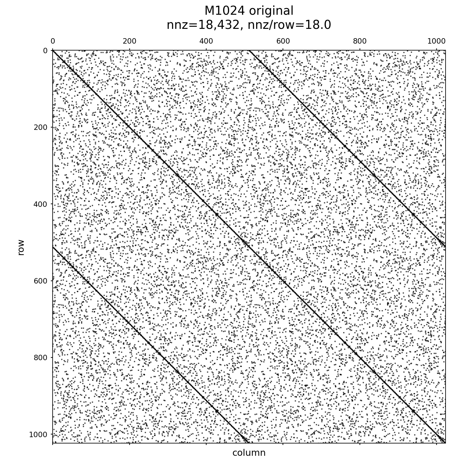
The matrix \(M\) constructed like above looks like the following, structurally:

you can visually get an idea for the expander structure by attempting a reordering like Reverse Cuthill-McKee (RCM) which attempts to move nonzeros into a band:

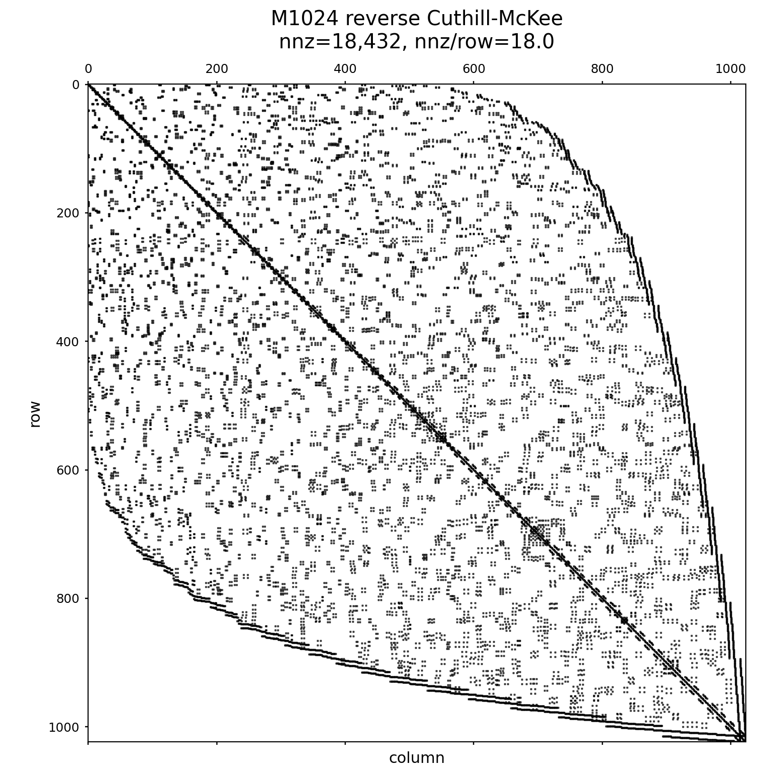
The RCM ordering doesn’t prove anything about the hardness of this system, but it is one useful datapoint and it is easy to visualize.

What I did next was the following, for both \( A_0 \) and \( M \) for different matrix sizes

1. I solved a system with CHOLMOD and reported the best achieved fill reduction after trying all available methods
2. I solved a system with Conjugate Gradients and reported number of iterations
3. I computed the resulting bandwidth after RCM reordering
4. I computed the “equivalent bandwidth” which is the bandwidth of a hypothetical matrix of the same size that would take the same memory as CHOLMOD’s computed \(L\) factor

I present a table for these below. The examples were chosen so that the resulting system would have \( \kappa(M) = 1e9 \)

The main things to look for are that CG takes essentially \(0.5n\) iterations on the lifted matrices, the fill grows rapidly with problem size, and RCM still leaves a very large bandwidth.

The trend above shows constant row sparsity, slow convergence for unpreconditioned CG, and approximately quadratic factor storage over these sizes. The number of CG iterations is \( \frac{1}{2}n \) in all these examples. Once the planted Chebyshev modes are resolved, it only has comparatively little work remaining for the original modes.

Potential Mitigations

Most solver libraries which only have access to the underlying sparse matrix and perhaps a few hints from the user (e.g. SPD, stencil structure, etc.) will not have preprocessing that can detect the block structure from the above matrix. But it is feasible that this structure could be detected, and the block orthogonal decomposition could be undone and the Chebyshev modes explicitly deflated away. We could achieve this by vertex matching algorithms since \( A_0 \) is replicated in a fairly straightforward block form into \( M \).

To obscure this, the \(D \) matrix could instead be a sparse SPD tridiagonal matrix constructed to have the desired spectrum. This introduces more nonzeros into \(M \) and makes simple vertex matching less useful. More generally, the block form here is just the simplest version of the adversarial idea.

Discussion

After removing the constant nullspace, fixed-degree expander graph Laplacians have a spectral gap and can be handled well by Krylov methods. The counterexample here is designed to show that favorable CG behavior is not a fundamental property of every sparse SPD matrix whose graph has expander-like structure: numerical values can plant a much less favorable spectrum even while the structural graph remains sparse.