Here I derive the elimination tree for the right-looking sparse Cholesky algorithm, computing A = LL^T for a lower triangular L and sparse symmetric positive definite A. Elimination trees also appear throughout sparse LU and QR software, though those factorizations require some additional machinery. For Cholesky, the tree tells us how to recover the structural fill pattern of L and compactly represents dependencies among factor columns. Traditionally this concept is often presented through sparse triangular solves used as building blocks for Cholesky. I wanted to instead work directly from a Cholesky factorization, which is what I do below.
Suppose at first we start with the plain dense right-looking Cholesky algorithm in pseudocode below:
// Input:  symmetric positive definite A, assigned to an output matrix L
// Output: lower triangular part of L is such that A = LL^T

for (int k = 0; k < n; ++k) {
    // 1. Factor the pivot
    L[k][k] = sqrt(L[k][k]);

    // 2. Scale the column below the pivot
    for (int i = k + 1; i < n; ++i) {
        L[i][k] /= L[k][k];
    }

    // 3. Right-looking rank-1 update of trailing matrix
    //    Note that it is only this step which will create fill-in.
    for (int j = k + 1; j < n; ++j) {
        for (int i = j; i < n; ++i) {   // lower triangle only
            L[i][j] -= L[i][k] * L[j][k];
        }
    }
}
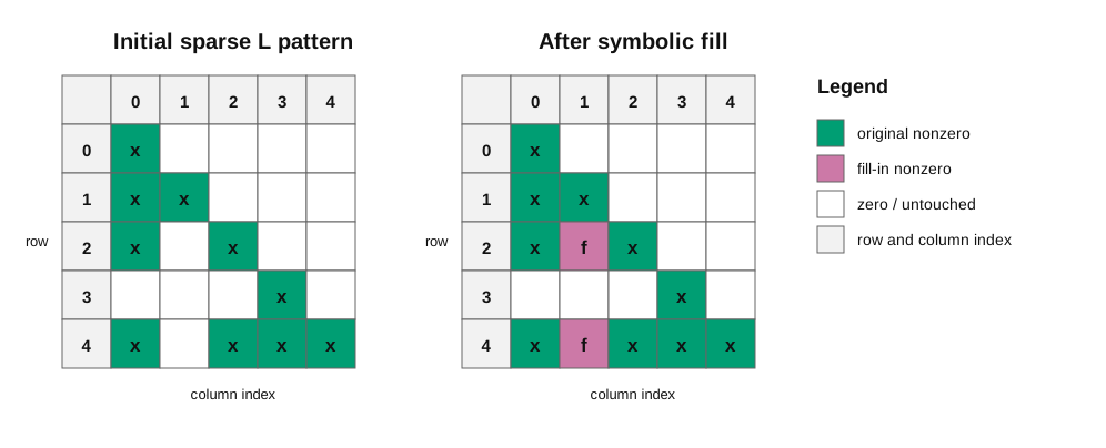
The implied order and loop structure results in a task DAG. In the event that A is sparse it turns out that the DAG as well as the implied structural fill-in from step (3) can be determined from the initial nonzero pattern of A and a simple tree data structure, known as the Cholesky elimination tree. Here and below I mean structural nonzeros, ignoring exact numerical cancellation. I will illustrate with a simple 5x5 matrix (only showing the lower triangular part to make it easier to read)
Terminology note: in sparse QR and other unsymmetric settings, the phrase column elimination tree often refers to the elimination tree of A^T A. Here A is already symmetric positive definite, so the tree derived below is the elimination tree of A itself, expressed as dependencies among columns of L.
Taking the above sparse matrix we get

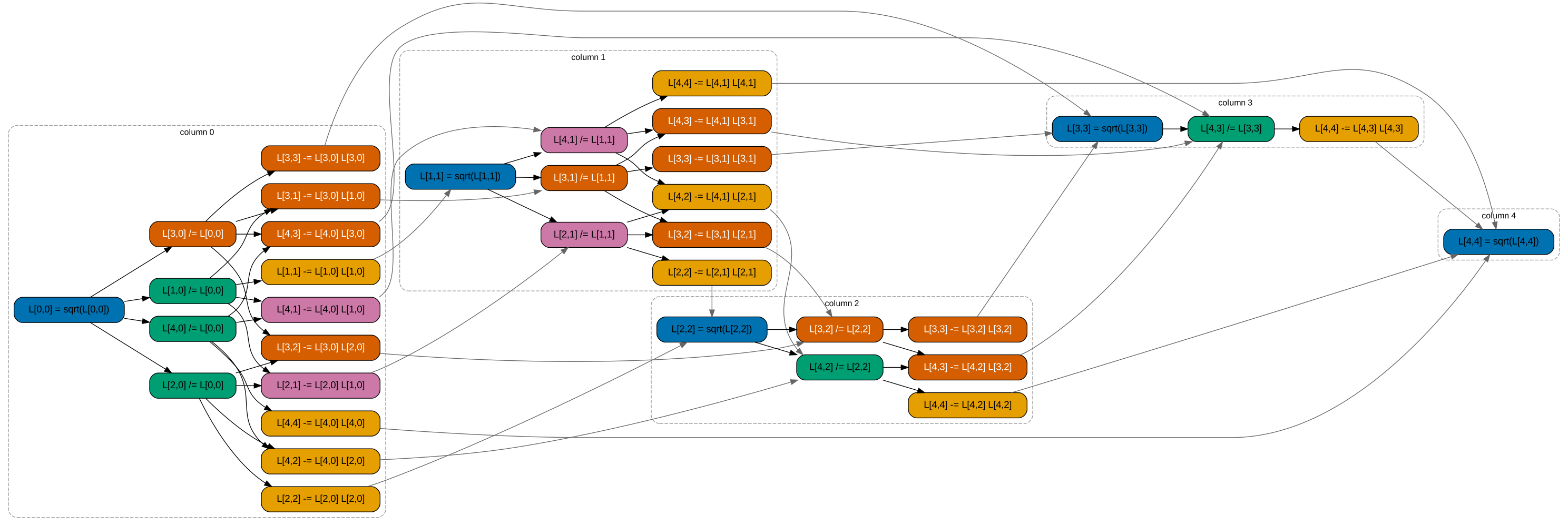
As expected, because A is sparse there are some operations here that we never need to do. If we prune these we get a much smaller graph.
Note the column grouping here doesn’t serve a practical purpose yet, but we may interpret a column group as meaning “when we have completed all operations in a column group i, no future operation references column i”.
Eliminating all unnecessary operations we get the following
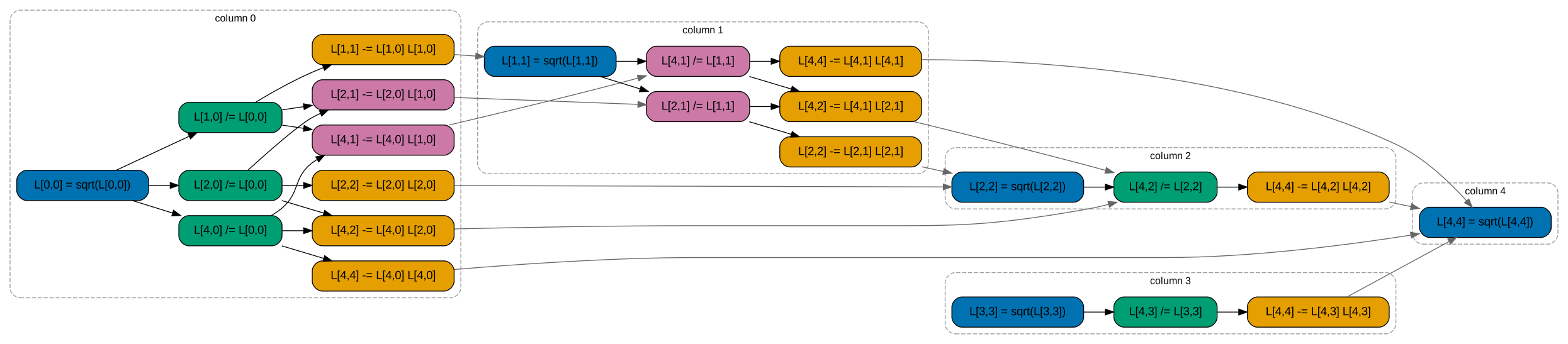
This pruned graph tells us every scalar operation in this particular right-looking Cholesky factorization. But in order to determine this graph I had to do a dense factorization and then prune the unnecessary calculations.
It turns out, however, that there is a simple O(n)-storage data structure which, when combined with the initial nonzero pattern of A, can quickly tell us the final structural fill pattern and the column-level dependencies. This is the Cholesky elimination tree; constructing and using it still takes work proportional to the sparse pattern traversed, not merely O(n) time in general.
Recalling step (3) from our dense Cholesky factorization
// 3. Right-looking rank-1 update of trailing matrix
//    Note that it is only this step which will create fill-in.
for (int j = k + 1; j < n; ++j) {
    for (int i = j; i < n; ++i) {   // lower triangle only
        L[i][j] -= L[i][k] * L[j][k];
    }
}
It tells us a key structural fact: if k < j <= i, and L[i][k] and L[j][k] are structurally nonzero, then L[i][j] is structurally nonzero.
Now when we look at the pruned task graph we can see some implied column dependencies like 0->1 and 0->2. Since 0 has two “parents” this is a DAG pattern rather than a tree. But the above structural rule tells us that 0->2 is a redundant edge because 0->1 necessarily means L[1,0]!=0, and 0->2 necessarily means L[2,0]!=0, and thus we must have L[2,1]!=0, and so there is an implied edge 1->2, and it is redundant information that 0->2 because we must proceed from 0->1 first anyway. If we retain only the nearest later dependency of each column, the result is an elimination tree—or, for a disconnected pattern, an elimination forest:
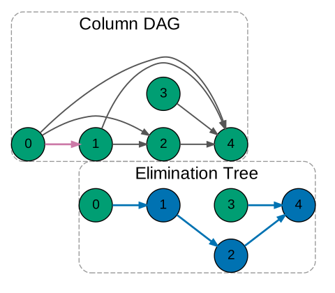
The elimination tree tells us how to generate the structural fill pattern of L from the initial nonzero pattern of A and the rule above.
I will defer calculation of the elimination tree to the end of this post and show now how we can use the elimination tree encoded as a parents array:
// Input:
//   n
//   A_row[i]      : original lower-triangular row pattern of A
//   parent[k]     : elimination tree parent of k, or -1
//   mark[k]       : caller-allocated scratch array of length n
//
// Output:
//   L_col[k]      : row indices i >= k for which L[i][k] exists
//
// Scratch:
//   mark[k] is overwritten.

void symbolic_cholesky(
    int n,
    int** A_row,
    int* A_row_len,
    int* parent,
    int* mark,
    vector_int* L_col
) {
    for (int k = 0; k < n; ++k) {
        mark[k] = -1;
        vector_clear(&L_col[k]);

        // Include the diagonal.
        vector_push(&L_col[k], k);
    }

    for (int i = 0; i < n; ++i) {
        for (int p = 0; p < A_row_len[i]; ++p) {
            int k = A_row[i][p]; // base nonzero A[i][k], k < i

            while (k != -1 && k < i && mark[k] != i) {
                mark[k] = i;

                // The tree path says L[i][k] exists.
                vector_push(&L_col[k], i);

                k = parent[k];
            }
        }
    }
}
Once we have the nonzero pattern of L writing the numeric factorization follows straightforwardly from the dense algorithm outline, using appropriate sparse matrix data structures. The key step is where fill-in is introduced, which I show in pseudo-c below
for (int j in L_col[k]) {
    if (j <= k) continue;

    for (int i in L_col[k]) {
        if (i < j) continue;

        L[i][j] -= L[i][k] * L[j][k];
    }
}
and since we precomputed the nonzero pattern we need not check if those numerical entries exist or not, they will have been preallocated.
The elimination tree is essentially:
parents[k] = min {j>k s.t. L[j,k]!=0}
To compute the elimination tree using only the starting nonzeros of A without excessive extra work we need to incrementally build parents. This means for each r we need to try and find the path to r in this tree.
So if we iterate through rows of A in order and then look at the column ids we get a candidate path c-> ... -> r. We save that c->r in ancestors[c] and iterate up ancestors until we found a column we have not yet matched, then that column’s parent becomes r, because we are iterating rows in order we can not find a smaller r.
In pseudo-C below:
// Compute the Cholesky elimination tree.
//
// Input:
//   n
//   A_row[r]      : columns c < r where A[r,c] is structurally nonzero
//   A_row_len[r]  : number of such columns in row r
//
// Output:
//   parent[k]     : parent of column k in the elimination tree,
//                   or -1 if k is a root
//
// Scratch:
//   ancestor[k]   : caller-owned scratch array of length n
//
// Sentinel:
//   -1 means "no parent / no ancestor has been assigned yet"

void compute_elimination_tree(
    int n,
    int** A_row,
    int* A_row_len,
    int* parent,
    int* ancestor
) {
    for (int k = 0; k < n; ++k) {
        parent[k] = -1;
        ancestor[k] = -1;
    }

    for (int r = 0; r < n; ++r) {
        for (int p = 0; p < A_row_len[r]; ++p) {
            int c = A_row[r][p]; // A[r,c] exists, with c < r

            // A[r,c] gives the ancestor constraint:
            //
            //     c -> ... -> r
            //
            // Walk upward from c through the paths already discovered.
            int v = c;

            while (v != -1 && v < r) {
                int next = ancestor[v];

                // Record that while processing row r, v has been
                // connected upward to r.
                ancestor[v] = r;

                if (next == -1) {
                    // This path stopped at v. Since rows are processed
                    // in increasing order, r is the first later row that
                    // needs v as an ancestor, so r is parent[v].
                    parent[v] = r;
                    break;
                }

                // Continue walking the previously discovered path.
                v = next;
            }
        }
    }
}
The presentation of elimination trees often involves some preliminary graph theory that always felt a little detached from the linear algebra. My aim here was not to replace the graph theory, but to make it more grounded in the underlying algorithm. I proceeded directly from the right-looking Cholesky factorization to a task DAG, pruned that DAG, and then showed that the structural rule implied by step (3) of the algorithm results in a compressed representation of the task DAG, and that compressed representation happens to be a tree.