In a recent post I gave intuition for the sparse Cholesky elimination tree by appealing to the task DAG and showed how it could be compressed into a tree in the sparse case. That post also showed how to use and compute the tree. Here I take a narrower and more conventional route: I start from a naive symbolic translation of right-looking Cholesky, identify the structural work it repeats, and show how retaining only the first later row affected by each factor column naturally produces the elimination tree.
Throughout, A is an n x n symmetric positive definite matrix in a fixed ordering, and A = LL^T. I store lower-triangular structural patterns by row, include every diagonal entry, and ignore exact numerical cancellation. Thus a “nonzero” below means a structural nonzero: an entry for which storage and work must be reserved even if a special choice of numerical values would make the computed entry vanish.
The elimination tree is a succinct O(n) data structure. Combined with the original nonzero pattern of A, it permits rapid queries about the structural pattern of L without storing that entire pattern. A symbolic factorization can explicitly enumerate all nonzeros of L, but it does not have to: it might instead compute counts, storage requirements, or other structural information directly from the tree. For simplicity I begin by explicitly materializing L. That operation is necessarily sensitive to nnz(L); computing the tree itself will not require enumerating the filled factor.
A Cholesky symbolic factorization analyzes the pattern, storage, and work required for L. One possible output is an explicit sparse pattern for the factor, which is the approach I take first. To begin, here is right-looking dense Cholesky:
import numpy as np


def dense_L(A):
    # Work on a floating-point copy. Only the returned lower triangle
    # contains the factor.
    A = np.array(A, dtype=float, copy=True)
    n_rows, n_cols = A.shape
    assert n_rows == n_cols
    n = n_rows

    for i in range(n):
        assert A[i, i] > 0.0

        # Factor the diagonal.
        A[i, i] = np.sqrt(A[i, i])

        # Scale column i below the diagonal.
        for row in range(i + 1, n):
            A[row, i] = A[row, i] / A[i, i]

        # Right-looking rank-one update of the trailing lower triangle.
        # This is where structural fill can occur.
        for row in range(i + 1, n):
            for col in range(i + 1, row + 1):
                A[row, col] -= A[row, i] * A[col, i]

    return np.tril(A)
For the symbolic routines below, A[row] is a set containing the lower-triangular structural column indices in row, including row itself. Every key from 0 through n - 1 is present. I use the same representation for L. Following the rank-one update above gives a simple way to compute the structural pattern of L, since that update is the only place where new entries can be introduced:
def symbolic_L_naive(A, n):
    # All structural entries of A are structural entries of L.
    # Copy each set so the input pattern is not modified.
    L = {row: set(A[row]) for row in range(n)}

    for i in range(n):
        # Find rows below the diagonal whose pattern contains column i.
        column_rows = [
            row
            for row in range(i + 1, n)
            if i in L[row]
        ]

        # Apply the full structural rank-one update.
        for row in column_rows:
            for col in column_rows:
                if col <= row:
                    L[row].add(col)

    return L
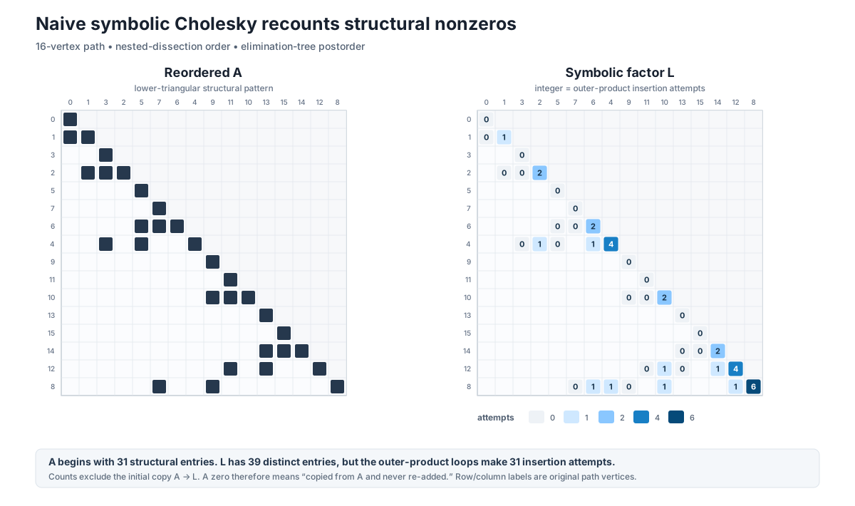
Because L[row] is a set, the routine above returns each structural entry only once. It nevertheless calls add repeatedly for entries that are already present. The figure below illustrates this for a 16-vertex path in nested-dissection order followed by elimination-tree postorder. The row and column labels are the original path vertices.
The lower triangle of A begins with 31 structural entries, while L has 39, so the factor contains only 8 new filled entries. After the initial copy from A to L, however, the full rank-one loops make 31 insertion attempts. Thus 23 attempts do not create a new distinct entry.
To see how this work can be deferred, suppose column i of L contains entries at rows p < q < r < s below the diagonal. Ignoring the diagonal entries, which already exist structurally, its update can introduce
L[q, p], L[r, p], L[s, p],
L[r, q], L[s, q],
L[s, r].
The naive routine also attempts to insert L[p, p], L[q, q], L[r, r], and L[s, s]; those diagonal attempts are included in the figure. For the off-diagonal pattern, it is enough at this step to insert only
L[q, p], L[r, p], L[s, p].
Those entries make q, r, and s appear in column p. When column p is processed, the same rule inserts the entries involving its first later row; subsequent columns continue the process. In this way the remaining structural entries are generated when they are first needed rather than all at once:
def symbolic_L_v2(A, n):
    L = {row: set(A[row]) for row in range(n)}

    for i in range(n):
        # Find rows below the diagonal whose pattern contains column i.
        column_rows = [
            row
            for row in range(i + 1, n)
            if i in L[row]
        ]

        # A root column has no later structural row.
        if not column_rows:
            continue

        # Retain only entries involving the first later row.
        p = column_rows[0]
        for row in column_rows[1:]:
            L[row].add(p)

    return L
This removes the full pairwise insertion loop, but it still constructs column_rows from the evolving pattern of L for every column. The quantity p, however, is exactly the piece of information retained by the elimination tree.
Intuitively, p = column_rows[0] is the first later row touched by column i during the Cholesky factorization. More precisely, define
parent[i] = min {j > i : L[j, i] is structurally nonzero}.
If that set is empty, column i is a root and parent[i] = None. Every nonroot satisfies i < parent[i], so the parent array cannot contain a cycle. It describes a tree when the pattern is irreducible and a forest for a reducible or block-diagonal pattern.
This definition gives a useful structural rule directly from the propagation above. Suppose L[i, k] is structurally nonzero with k < i, and let p = parent[k]. Since p is the first later row in column k, either p == i, or p < i and the first-row-only propagation inserts L[i, p]. Repeating the same argument from p gives
k -> parent[k] -> parent[parent[k]] -> ... -> i.
Thus every structural entry L[i, k] says that i is an ancestor of k. In particular this is true for every original entry A[i, k], since the structural pattern of A is copied into L. Row i of L can therefore be recovered from {i} together with the parent paths beginning at the off-diagonal column indices stored in A[i], stopping when those paths reach i.
def symbolic_L_etree(A, parent, n):
    L = {i: {i} for i in range(n)}
    mark = [-1] * n

    for i in range(n):
        for k in A[i]:
            if k >= i:
                continue

            node = k
            while (
                node is not None
                and node < i
                and mark[node] != i
            ):
                mark[node] = i
                L[i].add(node)
                node = parent[node]

            if node is None or node > i:
                raise ValueError("parent is inconsistent with A")

    return L
The marker is important here because different original entries in A[i] can lead into the same parent path. Once a node is marked for row i, the remainder of that path has already been added to L[i], so it need not be traversed again. There is no analogous collection of separate paths in symbolic_L_v2: that routine materializes each current factor column and propagates it once. The marker makes the etree version output-sensitive, with work proportional to nnz(A) + nnz(L) when it explicitly constructs the full pattern.
The elimination tree has now simplified the computation of L, but I have not yet shown how to compute parent without first constructing L. That is the particularly useful compression: the parent array can be obtained from A alone and then used for symbolic queries that need not enumerate every entry of the filled factor.
The reach argument above also tells us how to build parent. Process the rows of A in increasing order. When row i is reached, every parent assigned so far came from an earlier row and therefore has an index less than or equal to i. For every structural entry A[i, k] with k < i, row i must be an ancestor of k.
Start at k and follow the parent links already discovered. If the path reaches i, that constraint has already been satisfied. If it instead reaches a node with no parent, then i becomes that node’s parent. Because rows are processed in increasing order, i is the first and therefore smallest later row that can take that role:
def elimination_tree_uncompressed(A, n):
    parent = [None] * n

    for i in range(n):
        for k in A[i]:
            if k >= i:
                continue

            node = k

            while node != i:
                assert node < i

                if parent[node] is None:
                    parent[node] = i
                    break

                node = parent[node]

    return parent
This is the uncompressed algorithm used in my interactive elimination-tree trace. It does not enumerate L, but different entries of A can make it walk the same partial parent path repeatedly. A separate scratch array can compress those traversals.
Here parent remains the final elimination-tree output. ancestor is only a temporary jump structure: when a node is visited while processing row i, its scratch link is redirected toward i. A later traversal can then skip the portion of the path already processed:
def elimination_tree_path_compressed(A, n):
    parent = [None] * n
    ancestor = [None] * n

    for i in range(n):
        for k in A[i]:
            if k >= i:
                continue

            node = k

            while node is not None and node < i:
                next_node = ancestor[node]

                # Compress this traversal path toward i
                ancestor[node] = i

                # No earlier row established a path above this node.
                if next_node is None:
                    parent[node] = i

                node = next_node

    return parent
This implementation uses path compression without balancing. Its worst-case time is O(nnz(A) log n), with O(n) additional storage, and the bound does not contain nnz(L) because the filled factor is never enumerated. A balanced union-find implementation can improve the logarithmic factor to an inverse-Ackermann factor, but it requires extra rank and representative bookkeeping that does not add much to the fill-in argument here. These bounds are discussed in Joseph W. H. Liu, “The Role of Elimination Trees in Sparse Factorization,” Section 5.
Here is a small pattern with two filled entries. Running each route makes the equivalence explicit:
A = {
    0: {0},
    1: {0, 1},
    2: {0, 2},
    3: {1, 3},
    4: {2, 3, 4},
}
n = len(A)

L_reference = symbolic_L_naive(A, n)
L_deferred = symbolic_L_v2(A, n)
parent = elimination_tree_path_compressed(A, n)
L_reach = symbolic_L_etree(A, parent, n)

assert parent == [1, 2, 3, 4, None]
assert L_reference == {
    0: {0},
    1: {0, 1},
    2: {0, 1, 2},
    3: {1, 2, 3},
    4: {2, 3, 4},
}
assert L_deferred == L_reference
assert L_reach == L_reference
The naive rank-one propagation, the first-row-only propagation, and the parent-path traversal all produce the same structural factor. The difference is which information each method retains and how much already-known structure it revisits.
Starting from the dense right-looking update, the most direct symbolic factorization attempts to insert every structural pair produced by each factor column. Most of that work can be deferred: retaining entries involving only the first later row is enough for subsequent columns to propagate the rest. That first later row is the elimination-tree parent.
The resulting O(n) parent array does not by itself enumerate L, but together with the pattern of A it contains enough information to recover L by parent-path reach. Explicitly recovering the entire pattern remains output-sensitive in nnz(L); computing the tree or answering more compact symbolic questions need not expand that output.
There is a parallel graph-theoretic expression of the same argument. The evolving symbolic factor can be viewed as an elimination graph, and quotient-graph representations compress its updates and are useful in fill-reducing orderings such as approximate minimum degree. I have intentionally deferred that language here, not because it is less correct, but because carrying the matrix and graph terminology in parallel would distract from the core fill-in logic that produces the tree.